Dimensional Analysis and Similitude: Dimensional Analysis
Dimensional
Analysis and Similitude
Many problems of interest in fluid mechanics cannot be solved using the integral and/or differential equations. Wind motions around a football stadium, the air flow around the deflector on a semitruck, the wave motion around a pier or a ship, and air flow around aircraft are all examples of problems which are studied in the laboratory with the use of models. A laboratory study with the use of models is very expensive, however, and to minimize the cost, dimensionless parameters are used. In fact, such parameters are also used in numerical studies for the same reason.
Once an analysis is done on a model in the laboratory and all quantities of interest are measured, it is necessary to predict those same quantities on the prototype, such as the power generated by a large wind machine from measurements on a
much smaller model. Similitude is the study that allows us to predict the quantities to be expected on a prototype from measurements on a model. This will be done after our study of dimensional analysis that guides the model study.
6.1 Dimensional Analysis
Dimensionless parameters are obtained using a method called dimensional analysis. It is based on the idea of dimensional homogeneity: all terms in an equation must have the same dimensions. By simply using this idea, we can minimize the number of parameters needed in an experimental or analytical analysis, as will be shown. Any equation can be expressed in terms of dimensionless parameters simply by dividing each term by one of the other terms. For example, consider Bernoulli’s equation,

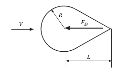
Let’s use an example to demonstrate the usefulness of dimensional analysis. Suppose the drag force is desired on an object with a spherical front that is shaped as shown in Fig. 6.1. A study could be performed, the drag force measured for a

particular radius R and length L in a fluid with velocity V, viscosity m, and density r.Gravity is expected to not influence the force. This dependence of the drag force on the other variables would be written as
To present the results of an experimental study, the drag force could be plotted as a function of V for various values of the radius R holding all other variables fixed. Then a second plot could show the drag force for various values of L holding all other variables fixed, and so forth. The plots may resemble those of Fig. 6.2. To vary the viscosity holding the density fixed and then the density holding the viscos- ity fixed, would require a variety of fluids leading to a very complicated study, and perhaps an impossible study.
The actual relationship that would relate the drag force to the other variables could be expressed as a set of dimensionless parameters, much like those of Eq. (6.2), as

sveral values of R/L would then provide the results of the study.

Before we present the details of forming the dimensionless parameters of Eq. (6.4), let’s review the dimensions on quantities of interest in fluid mechanics. Many quantities have obvious dimensions but for some, the dimensions are not so obvious. There are only three basic dimensions, since Newton’s second law can be used to relate the basic dimensions. Using F, M, L, and T as the dimensions on force, mass, length, and time, we see that F = ma demands that the dimensions are related by

where the brackets mean “the dimensions of.” Note that the product RT does not introduce additional dimensions.
Table 6.1 has been included to aid in selecting the proper dimensions for quantities of interest. It will simplify the creation of the dimensionless parameters. The dimensions are displayed for the M-L-T system only, since that will be what is used in the solution to the problems in this chapter. The same results would be obtained using the F-L-T system, should that system be selected.
The Buckingham p theorem is used to create the dimensionless parameters, given
a functional relationship such as that of Eq. (6.3). Write the primary variable of interest as a general function, such as
where n is the total number of variables. If m is the number of basic dimensions, usually 3, the Buckingham p theorem demands that (n − m) dimensionless groups of variables, the p terms, are related by
Table 6.1 Symbols and Dimensions of Quantities of Interest Using the M-L-T System

The steps that are followed when applying the Buckingham p theorem are:
1. Write the dependent variable as a function of the (n – 1) independent variables. This step requires knowledge of the phenomenon being studied. All variables that influence the dependent variable must be included and all variables that do not influence the dependent variable should not be included. In most problems, this relationship will be given.
2. Identify the m repeating variables that are combined with the remaining variables to form the p terms. The m variables must include all the basic dimensions present in the n variables of the functional relationship, but they must not form a dimensionless p term by themselves. Note that an angle is dimensionless, so it is not a candidate to be a repeating variable.
3. Combine each of the (n – m) variables with the repeating variables to form the p terms.
4. Write the p term containing the dependent variable as a function of the remaining p terms.
Step 3 is carried out by either inspection or by an algebraic procedure. The method of inspection will be used in an example. To demonstrate the algebraic procedure, let’s form a p term of the variables V, R, r, and m. This is written as


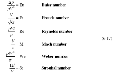
Finally, consider a very general functional relationship between a pressure change Δ p, a length l, a velocity V, gravity g, viscosity m, a density r, the speed of sound c, the surface tension s, and an angular velocity Ω. All of these variables
may not influence a particular problem, but it is interesting to observe the final relationship of dimensionless terms. Dimensional analysis, using V, l, and r as repeating variables provides the relationship
Each term that appears in this relationship is an important parameter in certain flow situations. The dimensionless term with its common name is listed as follows:

of fluid mechanics. The Euler number is of interest in most flows, the Froude number in flows with free surfaces in which gravity is significant (e.g., wave motion), the Reynolds number in flows in which viscous effects are important, the Mach number in compressible flows, the Weber number in flows affected by surface tension (e.g., sprays with droplets), and the Strouhal number in flows in which rotation or a periodic motion plays a role. Each of these numbers, with the exception of the Weber number (surface tension effects are of little engineering importance), will appear in flows studied in subsequent chapters. Note: The Froude number is often defined as V 2/ lg; this would not influence the solution to problems.
EXAMPLE 6.1
The pressure drop Δ p over a length L of pipe is assumed to depend on the aver- age velocity V, the pipe’s diameter D, the average height e of the roughness elements of the pipe wall, the fluid density r, and the fluid viscosity m. Write a relationship between the pressure drop and the other variables.
Solution
First, select the repeating variables. Do not select Δ p since that is the dependent variable. Select only one D, L, and e since they all have the dimensions of length. Select the variables that are thought2 to most influence the pressure drop: V, D, and r. Now, list the dimensions on each variable (refer to Table 6.1)
First, combine Δ p, V, D, and m into a p term. Since only Δ p and r have M as a dimension, they must occur as a ratio Δ p/r. That places T in the denominator so that V must be in the numerator so the T ’s cancel out. Finally, check out the L’s: there is L2 in the numerator so D2 must be in the denominator providing
The second p term is found by combining L with the three repeating variables
V, D, and r. Since both L and D have the dimension of length, the second p term is
The third p term results from combining e with the repeating variables. It has the dimension of length so the third p term is
The last p term is found by combining m with V, D, and r. Both m and r contain the dimension M demanding that they form the ratio r/m. This puts T in the numerator demanding that V goes in the numerator. This puts L in the denominator so that D must appear in the numerator. The last p term is then
The final expression relates the p terms as π1 = f (π 2 , π3 , π 4 ) or, using the variables,

EXAMPLE 6.2
The speed V of a weight when it hits the floor is assumed to depend on gravity g, the height h from which it was dropped, and the density r of the weight. Use dimensional analysis and write a relationship between the variables.
Solution
The dimensions of each variable are listed as
Since M occurs in only one variable, that variable r cannot be included in the relationship. The remaining three terms are combined to form a single p term; it is formed by observing that T occurs in only two of the variables, thus V 2 is in the numerator and g is in the denominator. The length dimension is then canceled by placing h in the denominator. The single p term is

A simple experiment would show that C = 2. We see that dimensional analysis rules out the possibility that the speed of free fall, neglecting viscous effects (e.g., drag), depends on the density of the material (or the weight).


